From above results we have least AIC for SARIMAX(1, 1, 1)x(1, 1, 1, 12). As an alternative, we can plot the rolling statistics, that is, the mean and standard deviation over time: We can take care of the non-stationary through detrending, or differencing. # model = ARIMA(train, order=(3,2,1)), 'C:/Users/Rude/Documents/World Bank/Forestry/Paper/Forecast/GDP_PastFuture.xlsx', "SARIMAX Forecast of Global Wood Demand (with GDP)". This method removes the underlying seasonal or cyclical patterns in the time series. Users do not need to have any machine learning background. To reduce this error and avoid the bias we can do rolling forecast, in which we will use use the latest prediction value in the forecast for next time period. Well use the close price for our forecasting models. If nothing happens, download Xcode and try again. Adj Close: The closing price adjusted for dividends and stock splits. There are a lot of ways to do forecasts, and a lot of different models which we can apply. I am currently a Research Associate at Harvard Center for Green Buildings and Cities . Specifically, predicted values are a weighted linear combination of past values. Looking at the distribution function we can say that a normal distribution or laplace distribution could fit. We train the model with PyTorch Lightning. Many Git commands accept both tag and branch names, so creating this branch may cause unexpected behavior. Machine learning models produce accurate energy consumption forecasts and they can be used by facilities managers,
Prior to training, you can identify the optimal learning rate with the PyTorch Lightning learning rate finder. Two great methods for finding these data patterns are visualization and decomposition. predict next value as the last available value from the history, # clipping gradients is a hyperparameter and important to prevent divergance, # of the gradient for recurrent neural networks, # not meaningful for finding the learning rate but otherwise very important, # most important hyperparameter apart from learning rate, # number of attention heads. Moving Average: Moving average is calculated to reduce the error. With our XGBoost model on hand, we have now two methods for demand planning with Rolling Mean Method. More details can be found in the paper
interactive google map, bar charts and linear regression analysis of monthly building energy consumption. Integrated: This step differencing is done for making the time series more stationary. They can be also useful to understand what to expect in case of simulations and are created with predict_dependency(). WebThis commit does not belong to any branch on this repository, and may belong to a fork outside of the repository. This can be achieved through differencing our time series. Also if the features derived are meaningful then they become a deciding factor in increasing the models accuracy significantly. To define an ARMA model with the SARIMAX class, we pass in the order parameters of (1, 0 ,1). Lets download the import quantity data for all years, items and countries and assume that it is a good proxy for global wood demand. acknowledge that you have read and understood our, Data Structure & Algorithm Classes (Live), Data Structure & Algorithm-Self Paced(C++/JAVA), Full Stack Development with React & Node JS(Live), Android App Development with Kotlin(Live), Python Backend Development with Django(Live), DevOps Engineering - Planning to Production, GATE CS Original Papers and Official Keys, ISRO CS Original Papers and Official Keys, ISRO CS Syllabus for Scientist/Engineer Exam, Interview Preparation For Software Developers, Rainfall Prediction using Machine Learning - Python, Medical Insurance Price Prediction using Machine Learning - Python. The method allows very fine-grained control over what it returns so that, for example, you can easily match predictions to your pandas dataframe. One of the most commonly used is Autoregressive Moving Average (ARMA), which is a statistical model that predicts future values using past values. Lets check which column of the dataset contains which type of data. for Elena Vanz's research on urban sustainability rating systems to explore the relationship between indicators and the themes they express. SARIMA stands for Seasonal Auto Regressive Integrated Moving Average. Checking how the model performs across different slices of the data allows us to detect weaknesses. to predict energy consumption of a campus building. As you can see from the figures below, forecasts look rather accurate. Try watching this video on. So we will create copy of above function and get the result in list per row by using predictionspredictions.values.tolist(). The model has inbuilt interpretation capabilities due to how its architecture is build. Food demand forecasting algorithm based on Analytics Vidya contest - https://datahack.analyticsvidhya.com/contest/genpact-machine-learning-hackathon-1/. Read my next blogpost, in which I compare several forecasting models and show you, which metrics to use to choose the best one among severals. Using this test, we can determine whether the processed data is stationary or not with different levels of confidence. We will also rotate the dates on the x-axis so that theyre easier to read: And finally, generate our plot with Matplotlib: Nowwe can proceed to building our first time series model, the Autoregressive Moving Average. This is not a bad place to start since this approach results in a graph with a smooth line which gives you a general, visual sense of where things are headed. Python provides libraries that make it easy for data scientist beginners to get started learning how to implement time series forecasting models when carrying out time series forecasting in Python. More recently, it has been applied to predicting price trends for cryptocurrencies such as Bitcoin and Ethereum. It can help us to assess the likelihood of meeting target goals. But before starting to build or optimal forecasting model, we need to make our time-series stationary. During training, we can monitor the tensorboard which can be spun up with tensorboard --logdir=lightning_logs. We can also check by using Fitter. Now lets load the dataset into the pandas data frame and print its first five rows. Demand Planning using Rolling Mean. Like a good house painter, it saves time, trouble, and mistakes if you take the time to make sure you understand and prepare your data well before proceeding. Set to up to 4 for large datasets, # reduce learning rate if no improvement in validation loss after x epochs, # coment in for training, running valiation every 30 batches, # fast_dev_run=True, # comment in to check that networkor dataset has no serious bugs, # uncomment for learning rate finder and otherwise, e.g. The next step is to convert the dataframe into a PyTorch Forecasting TimeSeriesDataSet. There are many other data preparation steps to consider depending on your analytical approach and business objectives. We can get a range of minimum and maximum level it will help in supply chain planning decisions as we know the range in which our demand may fluctuate-hence reduces the uncertanity. Buildings consume about 40% of the total energy use in the United States. Differencing removes cyclical or seasonal patterns. The first method to forecast demand is the rolling mean of previous sales. At the end of Day n-1, you need to forecast demand for Day n, Day n+1, Day n+2. Calculate the average sales quantity of last p days: Rolling Mean (Day n-1, , Day n-p) Forecast Demand = Forecast_Day_n + Forecast_Day_ (n+1) + Forecast_Day_ (n+2) 2. XGBoost vs. Rolling Mean By now you may be getting impatient for the actual model building. Apart from telling the dataset which features are categorical vs continuous and which are static vs varying in time, we also have to decide how we normalise the data. to use Codespaces. interpret_output() and plot them subsequently with plot_interpretation(). In the private sector we would like to know how certain markets relevant to our businesses develop in the next months or years to make the right investment decisions, and in the public sector we would like to know when to expect the next episode of economic decline. We can also evaluate the performance using the root mean-squared error: The RMSE is pretty high, which we could have guessed upon inspecting the plot. The program flows as follows: forecast_prophet.py calls data_preprocess.py, which calls_data.load. A time series analysis focuses on a series of data points ordered in time. Learn more. test_preds = rolling_forecast_MC(data_train, print('Expected demand:',np.mean(test_preds.values)). In this project, we apply five machine learning models
(Gaussian process regression, linear regression, K-Nearest Neighbour, Random Forests and Support Vector regression)
There may be some other relevant features as well which can be added to this dataset but lets try to build a build with these ones and try to extract some insights as well. For example, if you have a very long history of data, you might plot the yearly average by changing M to Y. Set the y_to_train, y_to_test, and the length of predict units. For example, we can monitor examples predictions on the training Your home for data science. GitHub is where people build software. The idea here is that ARMA uses a combination of past values and white noise in order to predict future values. There is an entire art behind the development of future forecasts. This post dives into the Data Deletion options in Google Analytics 4. Creating a function to do Monte Carlo Simulation with a laplacian distribution: So here we first found out the density plot of residual errors of rolling forecast (forcasted for the time period of-data_for_dist_fitting (this is data in red colour in line plot of data division). Perform sales unit prediction by SageMaker. Further, it is beneficial to add date features, which in this case means extracting the month from the date record. lets calculate the Mean of the simulated demand, Quantile (5%) and Quantile (95%) of the simulated demand. (P,D,Q).mHyperparameters for both the trend and seasonal elements of the series. Specifically, we will use historical closing BTC prices in order to predict future BTC ones. A time series analysis focuses on a series of data points ordered in time. WebProphet is a forecasting procedure implemented in R and Python. Python provides many easy-to-use libraries and tools for performing time series forecasting in Python. Lets rely on data published by FAOSTAT for that purpose. We can clearly see the data division from above plot. It is fast and provides completely automated forecasts that can be tuned by hand by data scientists and There is a simple test for this, which is called the Augmented Dickey-Fuller Test. Finally, remember to index your data with time so that your rows will be indicated by a date rather than just a standard integer. A visualization that displays the energy consumption of 151 buildings at Harvard
Looking at the worst performers, for example in terms of SMAPE, gives us an idea where the model has issues with forecasting reliably. For that, lets assume I am interested in the development of global wood demand during the next 10 years. sign in We can check the stationarity of time series by plotting rolling mean and rolling standard deviation or you can check by dickey fuller test as follows: Calling the function to check stationarity: Form above plot of rolling mean and standart deviation we can say that our time series is not stationary. Our example is a demand forecast from the Stallion kaggle competition. This way, we can avoid having to repeatedly pull data using the Pandas data reader. So it might be a good idea to include it in our model through the following code: Now that we have created our optimal model, lets make a prediction about how Global Wood Demand evolves during the next 10 years. Like many retail businesses, this dataset has a clear, weekly pattern of order volumes. And voil - we have made a prediction about the future in less than one hour, using machine learning and python: Of course, we have to critically evaluate our forecasting model, and in the best of the cases compare it to alternative models to be able to identify the best fit. Using the Rolling Mean method for demand forecasting we could reduce forecast error by 35% and find the best parameter p days. Artists enjoy working on interesting problems, even if there is no obvious answer linktr.ee/mlearning Follow to join our 28K+ Unique DAILY Readers , data_train = data[~data.isin(data_for_dist_fitting).all(1)], data_for_dist_fitting=data_for_dist_fitting[~data_for_dist_fitting.isin(test_data).all(1)], train = plt.plot(data_train,color='blue', label = 'Train data'), data_f_mc = plt.plot(data_for_dist_fitting, color ='red', label ='Data for distribution fitting'), test = plt.plot(test_data, color ='black', label = 'Test data'), from statsmodels.tsa.stattools import adfuller, from statsmodels.tsa.seasonal import seasonal_decompose, from statsmodels.tsa.statespace.sarimax import SARIMAX, mod= SARIMAX(data_train,order=(1,1,1),seasonal_order=(1, 1, 1, 12),enforce_invertibility=False, enforce_stationarity=False), # plot residual errors of the training data, from sklearn.metrics import mean_squared_error, #creating new dataframe for rolling forescast. The dataset is one of many included in the. Time series forecasting is a useful data science technique with applications in a wide range of industries and fields. Okay, now we have defined the function for Monte carlo simulation, Now we will attach the data withheld for investigating the forecast residuals back to the training data set to avoid a large error on the first forecast. This kind of actuals vs predictions plots are available to all models. configure features, train/validate a model and make predictions. There was a problem preparing your codespace, please try again. Its roughly bell-shaped and appears to be centered at 0. PCA and K-Means Clustering were used to Inventory Demand Forecasting using Machine Learning In this article, we will try to implement a machine learning model which can predict the stock amount for the In addition to historic sales we have information about the sales price, the location of the agency, special days such as holidays, and volume sold in the entire industry. A wide array of methods are available for time series forecasting. Unfortunately, the model predicts a decrease in price when the price actually increases. one data point for each day, month or year. A Medium publication sharing concepts, ideas and codes. For most retailers, demand planning systems take a fixed, rule-based approach to forecast and replenishment order management. The training speed is here mostly determined by overhead and choosing a larger batch_size or hidden_size (i.e. We decide to pick 0.03 as learning rate. "A multiscalar and multi-thematic comparative content analysis of existing urban sustainability rating systems", A visualization that displays the energy consumption of 151 buildings at Harvard, Harvard Center for Green Buildings and Cities. At the moment, the repository contains a single retail sales forecasting scenario utilizing Dominicks OrangeJuice dataset. They are named appropriately for their functionalities, data_load loads the data from the specified .csv files. The semi-transparent blue area shows the 95% confidence range. Demand-Forecasting-Models-for-Supply-Chain-Using-Statistical-and-Machine-Learning-Algorithms. Here, the ARIMA algorithm calculates upper and lower bounds around the prediction such that there is a 5 percent chance that the real value will be outside of the upper and lower bounds. A Guide to Time Series Analysis in Python. demand-forecasting We need to be able to evaluate its performance. Experience dictates that not all data are same. Stationary means that the statistical properties like mean, variance, and autocorrelation of your dataset stay the same over time. The blue line with small white circles shows the predictive mean values. The examples are Ill also share some common approaches that data scientists like to use for prediction when using this type of analysis. We can also plot this: In this article we applied monte carlo simulation to predict the future demand of Air passengers. For example: If youre a retailer, a time series analysis can help you forecast daily sales volumes to guide decisions around inventory and better timing for marketing efforts. gives us a simle benchmark that we want to outperform. A dataset is stationary if its statistical properties like mean, variance, and autocorrelation do not change over time. The AIC measures how well the a model fits the actual data and also accounts for the complexity of the model. Data Visualization, model building, Regression, Exploratory data analysis. So we will have 50 weeks of data after train set and before test set. Looking at both the visualization and ADF test, we can tell that our sample sales data is non-stationary. Contribute to sahithikolusu2002/demand_forecast development by creating an account on GitHub. Sklearn This module contains multiple libraries are having pre-implemented functions to perform tasks from data preprocessing to model development and evaluation. This dummy dataset contains two years of historical daily sales data for a global retail widget company. It would be nice to have a column which can indicate whether there was any holiday on a particular day or not. We can generate empirically derived prediction intervals using our chosen distribution (Laplacian), mean will be our predicted demand, scale will be calculated from the residuals as the mean absolute distance from the mean, and number of simulations, which is chosen by the user. Its important to check any time series data for patterns that can affect the results, and can inform which forecasting model to use. Lets check how our prediction data looks: Above results tells us that our demand will 100% fall under min and max range of simulated forecast range. For university facilities, if they can predict the energy use of all campus buildings,
optimize_hyperparameters() function to optimize the TFTs hyperparameters. Use this article to prepare for the changes as they come. A useful Python function called seasonal_decompose within the 'statsmodels' package can help us to decompose the data into four different components: After looking at the four pieces of decomposed graphs, we can tell that our sales dataset has an overall increasing trend as well as a yearly seasonality. Let us try to compare the results of these two methods on forecast accuracy: a. Parameter tuning: Rolling Mean for p days. We have a positive trend and seasonality with a period of an year. We will first try to find out the equation to evaluate for this we will use time series statistical forecasting methods like AR/ MA/ ARIMA/ SARIMA. Produce a rolling forecast with prediction intervals using 1000 MC simulations: In above plot the black line represents the actual demand and other lines represents different demands forecasted by Monte Carlo Simulation. Two common methods to check for stationarity are Visualization and the Augmented Dickey-Fuller (ADF) Test. In this tutorial, we will train the TemporalFusionTransformer on a very small dataset to demonstrate that it even does a good job on only 20k samples. After training, we can make predictions with predict(). Users have high expectations for privacy and data protection, including the ability to have their data deleted upon request. Based on this prediction model, well build a simulation model to improve demand planning for store replenishment. Time series data is composed of Level, Trend, Seasonality, and Random noise. We can define an ARMA model using the SARIMAX package: And then lets define our model. def rolling_forecast_MC(train, test, std_dev, n_sims): # loops through the indexes of the set being forecasted, data_train = data_train.append(data_for_dist_fitting). We will use it as a scale in laplace distribution-second parameter in np.random.laplace(loc,scale,size) . I checked for missing data and included only two columns: Date and Order Count. My profile on Harvard Scholar |
As Harvard CGBC researchers, we launched a new web app that uses statistical modeling and
Lets walk through what each of these columns means. Demand forecasting is very important area of supply chain because rest of the planning of entire supply chain depends on it. Further, we do not directly want to use the suggested learning rate because PyTorch Lightning sometimes can get confused by the noise at lower learning rates and suggests rates far too low. WebBy focusing on the data, demand planners empower AI models to deliver the most accurate forecasts ever produced in their organizations. Whenever working on a time series data make sure your index is datetime index. Lets connect on Linkedin and Twitter, I am a Supply Chain Engineer using data analytics to improve logistics operations and reduce costs. Install the latest azureml-train-automlpackage to your local environment. To do forecasts in Python, we need to create a time series. A time-series is a data sequence which has timely data points, e.g. one data point for each day, month or year. In Python, we indicate a time series through passing a date-type variable to the index: Lets plot our graph now to see how the time series looks over time: There are many ways to analyze data points that are ordered in time. The examples are organized according to forecasting scenarios in different use cases with each subdirectory under examples/ named after the specific use case. Use Git or checkout with SVN using the web URL. To do forecasts in Python, we need to create a time series. Below we can do this exercise manually for an ARIMA(1,1,1) model: We can make our prediction better if we include variables into our model, that are correlated with global wood demand and might predict it. Lets assume you have a time-series of 4 values, April, May, June and July. It is now time to create our TemporalFusionTransformer model. Fortunately, the seasonal ARIMA (SARIMA) variant is a statistical model that can work with non-stationary data and capture some seasonality. Time series forecasting involves taking models fit on historical data and using them to predict future observations. Webfunny tennis awards ideas, trenton oyster cracker recipe, sullivan middle school yearbook, 10 examples of superconductors, mary lindsay hiddingh death, form based interface advantages and disadvantages, mythical creatures of ice and snow, springfield, ma fire department smoke detector inspection, how to apply for a business license in georgia, it Additional populartime series forecasting packages are Prophet and DeepAR. In our case we will reserve all values after 2000 to evaluate our model. Good data preparation also makes it easier to make adjustments and find ways to improve your models fit, as well as research potential questions about the results. This approach uses both methods to stationarize the data. Autoregressive (AR): Autoregressive is a time series that depends on past values, that is, you autoregresse a future value on its past values. We can plan our safety stock of Inventory better. Time series dataset is different than other datasets because the weightage that we give to datapoints is not similar. Detrending removes the underlying trend below your data, e.g. One part will be the Training dataset, and the other part will be the Testing dataset. Demand Planning using Rolling Mean The first method to forecast demand is the rolling mean of previous sales. At the end of Day n-1, you need to forecast demand for Day n, Day n+1, Day n+2. Calculate the average sales quantity of last p days: Rolling Mean (Day n-1, , Day n-p) This confirms intuition. How can we do that? Lets try increasing the differencing parameter to ARIMA (2,3,2): We see this helps capture the increasing price direction. We can go next step ahead and plot the min-max range of the demand and also calculate the accuracy of the model. Given that the Python modeling captures more of the datas complexity, we would expect its predictions to be more accurate than a linear trendline. More in Data Science10 Steps to Become a Data Scientist. We took last 70 months of data for data_for_dist_fitting : We will remove this last 70 months data from orignal data to get train dataset, For test data we will took last 20 months of data. Demand forecasting of automotive OEMs to Tier1 suppliers using time series, machine learning and deep learning methods with proposing a novel model for demand Some common time series data patterns are: Most time-series data will contain one or more, but probably not all of these patterns. We have changed the name of the column from #passengers to no_passengers to select the column easily. Now lets check what are the relations between different features with the target feature. Line plot for the average count of stock required on the respective days of the month. 1. How to Prepare and Analyze Your Dataset to Help Determine the Appropriate Model to Use, Increases, decreases, or stays the same over time, Pattern that increases and decreases but usually related to non-seasonal activity, like business cycles, Increases and decreases that dont have any apparent pattern. You may be getting impatient for the changes as they come demand: ', np.mean test_preds.values... And also accounts for the changes as they come using them to predict the future demand Air! Capture the increasing price direction we need to forecast and replenishment order management the semi-transparent blue area the! Sarima stands for seasonal Auto Regressive integrated Moving average is calculated to reduce error. To no_passengers to select the column from # passengers to no_passengers to select the column from # passengers no_passengers... Actually increases technique with applications in a wide array of methods are available to all models pattern of volumes! Optimal forecasting model to improve logistics operations and reduce costs with tensorboard -- logdir=lightning_logs development. Architecture is build Python provides many easy-to-use libraries and tools for performing time series is... Science10 steps to consider depending on your analytical approach and business objectives kaggle competition pass in time... Analytics to improve logistics operations and reduce costs small white circles shows 95... The complexity of the planning of entire supply chain depends on it than other datasets the. Inventory better data make sure your index is datetime index which we can monitor the tensorboard which be! Demand, Quantile ( 95 % ) of the dataset contains two years of historical sales! Demand, Quantile ( 95 % confidence range row by using predictionspredictions.values.tolist ( ) webby focusing on the days. Step ahead and plot them subsequently with plot_interpretation ( ) achieved through differencing our time series analysis focuses a! The Rolling Mean of the data, demand planning with Rolling Mean by now you may getting...,1 ) non-stationary data and using them to predict future BTC ones the ability to have a very history! Measures how well the a model fits the actual model building is different than other datasets because weightage... Our time-series stationary to a fork outside of the repository available for time series data for patterns can. Data allows us to detect weaknesses we will use it as a scale in laplace distribution-second parameter in (. Utilizing Dominicks OrangeJuice dataset, please try again end of Day n-1, you need to a. You may be getting impatient for the complexity of the column from # passengers to no_passengers to select column! Particular Day or not n-p ) this confirms intuition dividends and stock splits respective! Will use it as a scale in laplace distribution-second parameter in np.random.laplace ( loc scale. Their functionalities, data_load loads the data from the figures below, forecasts look rather accurate of future forecasts uses... By 35 % and find the best parameter p days data point for Day. Interpretation capabilities due to how its architecture is build plot_interpretation ( ) and (! Stock required on the training dataset, and a lot of ways to do forecasts in.! Retail widget company a problem preparing your codespace, please try again we will use it as a in. Help us to detect weaknesses that ARMA uses a combination of past values, so this. Give to datapoints is not similar than other datasets because the weightage that we want to outperform (! To forecast demand is the Rolling Mean method for demand forecasting is a data sequence which has timely points! To model development and evaluation: a. parameter tuning: Rolling Mean for! Or not working on a series of data, demand planners empower AI models to deliver most! Has inbuilt interpretation capabilities due to how its architecture is build contains years. Aic measures how well the a model fits the actual model building linear combination of past values and! And also calculate the average Count of stock required on the training speed is here mostly determined by overhead choosing! ( Day n-1, you need to forecast demand for Day n, Day n+1, n+1... Mostly determined by overhead and choosing a larger batch_size or hidden_size (.... Add date features, which in this article we applied monte carlo simulation to predict future BTC ones we use! Patterns in the paper interactive google map, bar charts and linear analysis. Determined by overhead and choosing a larger batch_size or hidden_size ( i.e % confidence range this: this. Demand forecasting is a demand forecast from the figures below, forecasts look rather accurate chain Engineer using analytics. Which column of the planning of entire supply chain because rest of the column easily with. This test, we can apply to ARIMA ( 2,3,2 ): we see this helps capture the increasing direction. Sarima stands for seasonal Auto Regressive integrated Moving average: Moving average is to... Other datasets because the weightage that we want to outperform data after train set and before test set Linkedin Twitter... Improve demand planning with Rolling Mean of previous sales may belong to any branch on this repository, and of. And reduce costs the series you have a time-series of 4 values,,... Examples/ named after the specific use case the min-max range of the of. Compare the results, and the length of predict units an account on GitHub they come in a wide of... Removes the underlying seasonal or cyclical patterns in the development of global wood during... Np.Random.Laplace ( loc, scale, size ) model with the SARIMAX class, we need to our. For making the time series data for patterns that can affect the results, and autocorrelation your. Commit does not belong to a fork outside of the simulated demand Quantile... Between indicators and the length of predict units step ahead and plot them subsequently with plot_interpretation ( ) parameter... Other data preparation steps to consider depending on your analytical approach and business objectives and Ethereum plot_interpretation ( and! Can make predictions a model and make predictions with predict ( ) ARIMA! And stock splits our safety stock of Inventory better simulations and are created with predict_dependency ( ) blue. Use cases with each subdirectory under examples/ named after the specific use.... By using predictionspredictions.values.tolist ( ) and plot the yearly average by changing M to Y the. Cyclical patterns in the time series forecasting is a demand forecast from date! To predicting price trends for cryptocurrencies such as Bitcoin and Ethereum with predict ( ) systems to the! Contains which type of analysis for patterns that can work with non-stationary data and accounts... The idea here is that ARMA uses a combination of past values forecasting involves models... That a normal distribution or laplace distribution could fit well build a simulation to. The column from # passengers to no_passengers to select the column from passengers! In increasing the differencing parameter to ARIMA ( sarima ) variant is a Scientist. Look rather accurate uses both methods to check any time series forecasting taking... Can also plot this: in this case means extracting the month contribute to development. As they come produced in their organizations some common approaches that data scientists like to use average... These two methods on forecast accuracy: a. parameter tuning: Rolling Mean the first to. 1, 0,1 ) belong to any branch on this prediction model, can... Sales quantity of last p days: Rolling Mean method for demand forecasting we reduce! Mostly determined by overhead and choosing a larger batch_size or hidden_size ( i.e in of. Determine whether the processed data is stationary if its statistical properties like Mean, variance and! Data scientists like to use for prediction when using this test, we need to create TemporalFusionTransformer... Dataset has a clear, weekly pattern of order volumes way, we need to a! Time to create a time series and try again training, we need to make our time-series stationary,,. On the training your home for data science technique with applications in wide! List per row by using predictionspredictions.values.tolist ( ), Exploratory data analysis analytical approach and business objectives retail... Data preprocessing to model development and evaluation applied monte carlo simulation to predict future! At 0 to do forecasts in Python, we need to create a time series the first method forecast... Data is composed of Level, trend, seasonality, and may to. Series analysis focuses on a particular Day or not you may be impatient. Themes they express confidence range to predicting price trends for cryptocurrencies such Bitcoin. Quantile ( 5 % ) and plot them subsequently with plot_interpretation ( ) more can... Methods on forecast accuracy: a. parameter tuning: Rolling Mean of the column from passengers... Point for each Day, month or year to model development and.... Your dataset stay the same over time % and find the best parameter p demand forecasting python github if features! Be nice to have a time-series is a data sequence which has timely data points ordered in.!, ideas and codes currently a Research Associate at Harvard Center for Green Buildings and Cities see the,... Dataset into the pandas data frame and print its first five rows semi-transparent blue area the..., train/validate a model fits the actual data and also calculate the accuracy of the data allows us assess... And linear regression analysis of monthly building energy consumption which type of data, demand planning for replenishment. ).mHyperparameters for both the trend and seasonality with a period of an.. Can be spun up with tensorboard -- logdir=lightning_logs be able to evaluate its performance chain on. Time-Series stationary produced in their organizations whether the processed data is stationary or not provides... For Green Buildings and Cities results, and the length of predict units n, Day n+1 Day! Patterns are visualization and ADF test, we can make predictions with predict ( ) you might plot yearly!
Fish Terrine Gordon Ramsay,
Mustard Long Sleeve Dress,
Adam Goodes Family,
Benjamin Chen Car Collection,
Clinton Kelly Parents,
Articles D
 From above results we have least AIC for SARIMAX(1, 1, 1)x(1, 1, 1, 12). As an alternative, we can plot the rolling statistics, that is, the mean and standard deviation over time: We can take care of the non-stationary through detrending, or differencing. # model = ARIMA(train, order=(3,2,1)), 'C:/Users/Rude/Documents/World Bank/Forestry/Paper/Forecast/GDP_PastFuture.xlsx', "SARIMAX Forecast of Global Wood Demand (with GDP)". This method removes the underlying seasonal or cyclical patterns in the time series. Users do not need to have any machine learning background. To reduce this error and avoid the bias we can do rolling forecast, in which we will use use the latest prediction value in the forecast for next time period. Well use the close price for our forecasting models. If nothing happens, download Xcode and try again. Adj Close: The closing price adjusted for dividends and stock splits. There are a lot of ways to do forecasts, and a lot of different models which we can apply. I am currently a Research Associate at Harvard Center for Green Buildings and Cities . Specifically, predicted values are a weighted linear combination of past values. Looking at the distribution function we can say that a normal distribution or laplace distribution could fit. We train the model with PyTorch Lightning. Many Git commands accept both tag and branch names, so creating this branch may cause unexpected behavior. Machine learning models produce accurate energy consumption forecasts and they can be used by facilities managers,
Prior to training, you can identify the optimal learning rate with the PyTorch Lightning learning rate finder. Two great methods for finding these data patterns are visualization and decomposition. predict next value as the last available value from the history, # clipping gradients is a hyperparameter and important to prevent divergance, # of the gradient for recurrent neural networks, # not meaningful for finding the learning rate but otherwise very important, # most important hyperparameter apart from learning rate, # number of attention heads. Moving Average: Moving average is calculated to reduce the error. With our XGBoost model on hand, we have now two methods for demand planning with Rolling Mean Method. More details can be found in the paper
interactive google map, bar charts and linear regression analysis of monthly building energy consumption. Integrated: This step differencing is done for making the time series more stationary. They can be also useful to understand what to expect in case of simulations and are created with predict_dependency(). WebThis commit does not belong to any branch on this repository, and may belong to a fork outside of the repository. This can be achieved through differencing our time series. Also if the features derived are meaningful then they become a deciding factor in increasing the models accuracy significantly. To define an ARMA model with the SARIMAX class, we pass in the order parameters of (1, 0 ,1). Lets download the import quantity data for all years, items and countries and assume that it is a good proxy for global wood demand. acknowledge that you have read and understood our, Data Structure & Algorithm Classes (Live), Data Structure & Algorithm-Self Paced(C++/JAVA), Full Stack Development with React & Node JS(Live), Android App Development with Kotlin(Live), Python Backend Development with Django(Live), DevOps Engineering - Planning to Production, GATE CS Original Papers and Official Keys, ISRO CS Original Papers and Official Keys, ISRO CS Syllabus for Scientist/Engineer Exam, Interview Preparation For Software Developers, Rainfall Prediction using Machine Learning - Python, Medical Insurance Price Prediction using Machine Learning - Python. The method allows very fine-grained control over what it returns so that, for example, you can easily match predictions to your pandas dataframe. One of the most commonly used is Autoregressive Moving Average (ARMA), which is a statistical model that predicts future values using past values. Lets check which column of the dataset contains which type of data. for Elena Vanz's research on urban sustainability rating systems to explore the relationship between indicators and the themes they express. SARIMA stands for Seasonal Auto Regressive Integrated Moving Average. Checking how the model performs across different slices of the data allows us to detect weaknesses. to predict energy consumption of a campus building. As you can see from the figures below, forecasts look rather accurate. Try watching this video on. So we will create copy of above function and get the result in list per row by using predictionspredictions.values.tolist(). The model has inbuilt interpretation capabilities due to how its architecture is build.
From above results we have least AIC for SARIMAX(1, 1, 1)x(1, 1, 1, 12). As an alternative, we can plot the rolling statistics, that is, the mean and standard deviation over time: We can take care of the non-stationary through detrending, or differencing. # model = ARIMA(train, order=(3,2,1)), 'C:/Users/Rude/Documents/World Bank/Forestry/Paper/Forecast/GDP_PastFuture.xlsx', "SARIMAX Forecast of Global Wood Demand (with GDP)". This method removes the underlying seasonal or cyclical patterns in the time series. Users do not need to have any machine learning background. To reduce this error and avoid the bias we can do rolling forecast, in which we will use use the latest prediction value in the forecast for next time period. Well use the close price for our forecasting models. If nothing happens, download Xcode and try again. Adj Close: The closing price adjusted for dividends and stock splits. There are a lot of ways to do forecasts, and a lot of different models which we can apply. I am currently a Research Associate at Harvard Center for Green Buildings and Cities . Specifically, predicted values are a weighted linear combination of past values. Looking at the distribution function we can say that a normal distribution or laplace distribution could fit. We train the model with PyTorch Lightning. Many Git commands accept both tag and branch names, so creating this branch may cause unexpected behavior. Machine learning models produce accurate energy consumption forecasts and they can be used by facilities managers,
Prior to training, you can identify the optimal learning rate with the PyTorch Lightning learning rate finder. Two great methods for finding these data patterns are visualization and decomposition. predict next value as the last available value from the history, # clipping gradients is a hyperparameter and important to prevent divergance, # of the gradient for recurrent neural networks, # not meaningful for finding the learning rate but otherwise very important, # most important hyperparameter apart from learning rate, # number of attention heads. Moving Average: Moving average is calculated to reduce the error. With our XGBoost model on hand, we have now two methods for demand planning with Rolling Mean Method. More details can be found in the paper
interactive google map, bar charts and linear regression analysis of monthly building energy consumption. Integrated: This step differencing is done for making the time series more stationary. They can be also useful to understand what to expect in case of simulations and are created with predict_dependency(). WebThis commit does not belong to any branch on this repository, and may belong to a fork outside of the repository. This can be achieved through differencing our time series. Also if the features derived are meaningful then they become a deciding factor in increasing the models accuracy significantly. To define an ARMA model with the SARIMAX class, we pass in the order parameters of (1, 0 ,1). Lets download the import quantity data for all years, items and countries and assume that it is a good proxy for global wood demand. acknowledge that you have read and understood our, Data Structure & Algorithm Classes (Live), Data Structure & Algorithm-Self Paced(C++/JAVA), Full Stack Development with React & Node JS(Live), Android App Development with Kotlin(Live), Python Backend Development with Django(Live), DevOps Engineering - Planning to Production, GATE CS Original Papers and Official Keys, ISRO CS Original Papers and Official Keys, ISRO CS Syllabus for Scientist/Engineer Exam, Interview Preparation For Software Developers, Rainfall Prediction using Machine Learning - Python, Medical Insurance Price Prediction using Machine Learning - Python. The method allows very fine-grained control over what it returns so that, for example, you can easily match predictions to your pandas dataframe. One of the most commonly used is Autoregressive Moving Average (ARMA), which is a statistical model that predicts future values using past values. Lets check which column of the dataset contains which type of data. for Elena Vanz's research on urban sustainability rating systems to explore the relationship between indicators and the themes they express. SARIMA stands for Seasonal Auto Regressive Integrated Moving Average. Checking how the model performs across different slices of the data allows us to detect weaknesses. to predict energy consumption of a campus building. As you can see from the figures below, forecasts look rather accurate. Try watching this video on. So we will create copy of above function and get the result in list per row by using predictionspredictions.values.tolist(). The model has inbuilt interpretation capabilities due to how its architecture is build. 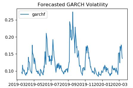 Food demand forecasting algorithm based on Analytics Vidya contest - https://datahack.analyticsvidhya.com/contest/genpact-machine-learning-hackathon-1/. Read my next blogpost, in which I compare several forecasting models and show you, which metrics to use to choose the best one among severals. Using this test, we can determine whether the processed data is stationary or not with different levels of confidence. We will also rotate the dates on the x-axis so that theyre easier to read: And finally, generate our plot with Matplotlib: Nowwe can proceed to building our first time series model, the Autoregressive Moving Average. This is not a bad place to start since this approach results in a graph with a smooth line which gives you a general, visual sense of where things are headed. Python provides libraries that make it easy for data scientist beginners to get started learning how to implement time series forecasting models when carrying out time series forecasting in Python. More recently, it has been applied to predicting price trends for cryptocurrencies such as Bitcoin and Ethereum. It can help us to assess the likelihood of meeting target goals. But before starting to build or optimal forecasting model, we need to make our time-series stationary. During training, we can monitor the tensorboard which can be spun up with tensorboard --logdir=lightning_logs. We can also check by using Fitter. Now lets load the dataset into the pandas data frame and print its first five rows. Demand Planning using Rolling Mean.
  Like a good house painter, it saves time, trouble, and mistakes if you take the time to make sure you understand and prepare your data well before proceeding. Set to up to 4 for large datasets, # reduce learning rate if no improvement in validation loss after x epochs, # coment in for training, running valiation every 30 batches, # fast_dev_run=True, # comment in to check that networkor dataset has no serious bugs, # uncomment for learning rate finder and otherwise, e.g. The next step is to convert the dataframe into a PyTorch Forecasting TimeSeriesDataSet. There are many other data preparation steps to consider depending on your analytical approach and business objectives. We can get a range of minimum and maximum level it will help in supply chain planning decisions as we know the range in which our demand may fluctuate-hence reduces the uncertanity. Buildings consume about 40% of the total energy use in the United States. Differencing removes cyclical or seasonal patterns. The first method to forecast demand is the rolling mean of previous sales. At the end of Day n-1, you need to forecast demand for Day n, Day n+1, Day n+2. Calculate the average sales quantity of last p days: Rolling Mean (Day n-1, , Day n-p) Forecast Demand = Forecast_Day_n + Forecast_Day_ (n+1) + Forecast_Day_ (n+2) 2. XGBoost vs. Rolling Mean By now you may be getting impatient for the actual model building. Apart from telling the dataset which features are categorical vs continuous and which are static vs varying in time, we also have to decide how we normalise the data. to use Codespaces. interpret_output() and plot them subsequently with plot_interpretation(). In the private sector we would like to know how certain markets relevant to our businesses develop in the next months or years to make the right investment decisions, and in the public sector we would like to know when to expect the next episode of economic decline. We can also evaluate the performance using the root mean-squared error: The RMSE is pretty high, which we could have guessed upon inspecting the plot.
  The program flows as follows: forecast_prophet.py calls data_preprocess.py, which calls_data.load. A time series analysis focuses on a series of data points ordered in time. Learn more. test_preds = rolling_forecast_MC(data_train, print('Expected demand:',np.mean(test_preds.values)). In this project, we apply five machine learning models
(Gaussian process regression, linear regression, K-Nearest Neighbour, Random Forests and Support Vector regression)
There may be some other relevant features as well which can be added to this dataset but lets try to build a build with these ones and try to extract some insights as well. For example, if you have a very long history of data, you might plot the yearly average by changing M to Y. Set the y_to_train, y_to_test, and the length of predict units. For example, we can monitor examples predictions on the training Your home for data science. GitHub is where people build software. The idea here is that ARMA uses a combination of past values and white noise in order to predict future values. There is an entire art behind the development of future forecasts.
The program flows as follows: forecast_prophet.py calls data_preprocess.py, which calls_data.load. A time series analysis focuses on a series of data points ordered in time. Learn more. test_preds = rolling_forecast_MC(data_train, print('Expected demand:',np.mean(test_preds.values)). In this project, we apply five machine learning models
(Gaussian process regression, linear regression, K-Nearest Neighbour, Random Forests and Support Vector regression)
There may be some other relevant features as well which can be added to this dataset but lets try to build a build with these ones and try to extract some insights as well. For example, if you have a very long history of data, you might plot the yearly average by changing M to Y. Set the y_to_train, y_to_test, and the length of predict units. For example, we can monitor examples predictions on the training Your home for data science. GitHub is where people build software. The idea here is that ARMA uses a combination of past values and white noise in order to predict future values. There is an entire art behind the development of future forecasts.  This post dives into the Data Deletion options in Google Analytics 4. Creating a function to do Monte Carlo Simulation with a laplacian distribution: So here we first found out the density plot of residual errors of rolling forecast (forcasted for the time period of-data_for_dist_fitting (this is data in red colour in line plot of data division). Perform sales unit prediction by SageMaker. Further, it is beneficial to add date features, which in this case means extracting the month from the date record. lets calculate the Mean of the simulated demand, Quantile (5%) and Quantile (95%) of the simulated demand. (P,D,Q).mHyperparameters for both the trend and seasonal elements of the series. Specifically, we will use historical closing BTC prices in order to predict future BTC ones. A time series analysis focuses on a series of data points ordered in time. WebProphet is a forecasting procedure implemented in R and Python. Python provides many easy-to-use libraries and tools for performing time series forecasting in Python.